Construction Detection using Satellite Images
Objective:
Localize and Identify the areas with possible under construction sites using satellite images.
Available Data :
- Satellite images for few areas (AOI).
- Each AOI image is capture for 3 months. Each of the above image is pan sharpend and cut into tiles of size 2km x 2km i.e., around 4000*4000 pixel each, considering each pixel translates to 50cm on the ground distance.
- Images clipped from the AOIs for buildings / sites under construction.
In Short:
- We have data for areas which probably have construction sites in them.
- For each area we have multiple images for different time periods each captured with gap of around a month’s time.
- Clipped satellite images for construction sites in different stages is available.
Introduction:
Given are the Satellite Images each spanning upto 400sq.kms taken 4 times over a period. The objective is to identify the locations where there is some kind of activity with respect to construction. Stated otherwise, we have to identify the locations where probably there is some building under construction. It is a non-trivial problem in the domain of sensory image analysis and requires knowledge in Computer Vision and Change Detection apart from usual sensory image analysis.
Challenges:
- The images captured over different time periods have been taken from different satellites, which introduces distortions in the images on overlapping. Overlaying two images from same site does not result into an exact overlap of the sites on the ground.
- Images captured are off-nadir images captured from different angles, which results in differences in image and footprint of buildings, houses or any other structures on the ground.
- In captured images, each pixel corresponds to roughly 50cm x 50cm on the ground distance, whereas in general a wall of a house is roughly maximum 30cm (12-13 inch) wide. So in general, it is tough to properly distinguish a wall on the ground using satellite images with lesser resolution.
- It is tough to distinguish between the different stages of the construction with just eyeballing the satellite images at concerned sites.
- Lack of labelled data for construction sites and different stages of construction.
Looking at the data available, we make a few rational assumptions for our experiments.
Assumptions:
- All construction sites will have similar surface features.
- The areas with construction sites will have a different image texture from any other kind of areas on the land.
- If observed over multiple time periods any structural change is captured as a prominent change in the sensory image values leading us to detecting the change.
- With the above assumption, upon initial study into the problem, it is concluded that we can attack the problem from 3 different directions. The 3 approaches leverage each kind of information(data) we have, which can be listed as below.
Approaches
- We know how does a construction site looks like from clipped image. – Template Matching
- We know that texture of a construction site is different from other kind of land usage. – Land Usage Classification
- Also as construction moves on a site there will be change observed on the site over time. – Change Detection
Approaches Explained:
I. Template Matching, Detailed Approach:
The approach involves matching the templates from clipped images for under construction sites with the tiles of each AOI to identify the other similar under construction sites. The methods used for the template matching are as follows:
- ORB
- SURF
- SIFT
- Root-SIFT
Based on experiments with each of the above techniques. Root-SIFT worked best for our problem.
To start with a mask using NDVI and Pantex is generated beforehand over the whole tile image which is to be used later. The tile images are then scanned over using a window function of size 400x400 pixels. In each window a segmentation, template matching and filtering of matched keypoints is carried out. More details are given below.
Step 0: Image Sharpening, Smoothing and Filtering: Images are sharpened and smoothened before using them for further processing. Some of the sharpening methods tried are Gaussian Blurring, 2D Kernel Sharpening (using various kernel sizes and values) and Bilateral Filtering. Sharpening using Gaussian Blur worked the best for the problem. Both templates and tile images are put through the above process to get better results in template matching.
Step 1: Segmentation:
Various segmentation techniques are tried to segment the windows of the tile images to localize the areas and clutser the matched keypoints. Some of them are :
Felzenshwalb Chan Vese Segmentation SLIC Watershed and Compact Watershed QuickShift Based on experiments Felzenswalb turned out to be optimum technique which yielded best results in reasonable time.
Step 2: Feature Descriptors Extraction and Matching:
Templates images of construction sites are collected from available clipped images which were manually collected from AOI1 and AOI2 earlier. Multiple experiments are done for matching template images to their respective clipped images using different algorithms to reach at best template matching technique for our use case.
Some of the facts observed during the above experimentation:
Root-SIFT with a FLANN based matcher worked best for matching template images with their respective clipped images.
On matching template images with other clipped images from the same class produced promising results (80% match) for column and brickwork but only satisfactory results(50-60% match) for excavation and foundation.
On matching template images with other clipped images from the other classs produced satisfactory results when the templates were picked from column and brickwork but not so promising results when templates from excavation and foundation are used. Features from column and brickwork matches with all the classes i.e., column, brickwork,excavation and foundation. But with features picked from excavation and foundation matched everywhere on the image and are not able to capture the site of construction. So we chose the brickwork and column templates for building our features in further processing.
On merging features from multiple templates and matching them over the images yielded better results than using individual templates separately. Merged features are clustered and cluster centers are chosen as representative descriptor features for template matching. From these features we chose only the features(cluster centers) whose cluster frequency lie between 20% to 80%. As the clusters below them would bring in artifacts which are particular to few images and clusters above 80% frequency will contain features which are very common and non-discriminatory. These medium frequency range features yielded better results with lower false positives and more relevant locations being matched.
A lot of descriptors are matched on the barren / shrub land, may be due to a lot of varying texture in those areas which is also a characteristic of sites under construction.
Step 3: Image Masking:
Pantex : A medium pass filter is used to generate a mask for areas which are lying in between the Fully completed built-up areas and fully non-builtup areas. Pantex index is not an upper bounded index and has maximum values for tiles varying somewhere between 1500 to 4000. Selelcting a proper threshold is a challenge in such scenario. We choose a lower threshold of 100 and upper threshold of 1000 to achieve a medium pass filter. Upon manual observation the result look satisfying as most of the fully builtup area, clearly non-built up areas is masked correctly, leaving a few areas with undesirable masking.
NDVI: Vegetation filter is applied to the remaining areas to remove any kind of vegetation form the tile images.
The above two masks are merged to get a final mask.
Step 4.1: First level Segment Filtering:
At first level the image is traversed in 400 by 400 pixels window. In each window the image is segmented using Felzenswalb method and Root-SIFT descriptors are matched to find the keypoints. Any keypoint occuring on the masks calculated above are filtered out and then only the segments which contain enough number of keypoints in them are selected.
This step is taken to increase the relevance of keypoints as keypoints occuring together in a single segments increase the relvance of that segment instead of another segments which has a sparse occurence of keypoints in it. Once we have selected the segments and their corresponding keypoints in each window, other keypoints are dropped from further consideration in the pipeline.
Step 4.2: Second level Segment Filtering:
Once we have collected the filtered keypoints from the step above. The tile image of 2km by 2km is again segmented using Compact Watershed method. Each segment is then classified into one of the four classes given as Barren, Vegetation, Under construction and Built-up area. Once classified the segments go through second level of filtering in which only the segments containing enough number of keypoints are selected. The classification features and process is described later.
II. Land Usage Classification, Detailed Approach:
2. Land Usage Classification:
This approach involves Land Usage classification using machine learning methods. We try to classifiy the kind of land usage in an image based on multiple texture features, which include:
- Haralick and GCLM features
- Pantex Index
- Lacunarity
- Texton
- LBP(Linear Binary Pattern)
- HOG (Histogram of Gradients)
- TAS (Threshold Adjacency Statistic)
Other kind of features calculated over pixel windows in different bands involve:
- Mean, Median, Mode, Min and Max
- Histogramic Features
- Distribution features such as Variance/SD, Skewness Kurtosis over each bands spectrum density
To carry out the classification we use the clipped images as our training dataset for under construction class and for other classes we clipped multiple images from the AOI1 and AOI2 tiles. These other classes include waterbody, barren land, completed building and farmlands. Some more of under construction sites are clipped from the AOI1/2 Images.
Unsupervised Classification:
An unsupervised classification model is trained for land classification using multiple features obtained through transformation of the image such as LAB, LUV transformation, HSV transformation and Ratio features. The results of the unsupervised classification are used in the supervised classification model in form of the density of each class in the concerned area being classified.
Supervised Classification
The results of the unsupervised classification are used in the supervised classification model in form of the density of each class in the concerned area being classified. An illustrative image is given below. Out of all the other features tried and tested LBP features at 3 different levels constitute the major features for training the XGB classification model. LBP features are calculated over rgb image and unsupervised class result to capture the contextual information captured in the unsupervised classification. Other features used are GLCM features. About 900 images from 4 different classes are used for training the model and an average precision of 90% and recall of 88% is achieved over the validation set.
III. Change Detection:
In this approach we try to find out the construction sites by calculating the changes in AOI tile Images over a period of time. Although the pre-requisite to the approach is that the images from different periods should have a perfect overlap on the cartographic grid. This above procedure involves Orthorectification and Coregisteration to make the images ready for Change Detection. Some of the change detection methods which are investigated include
- Change Vector Analysis(CVA),
- Multivariated Alteration Detection(MAD),
- Iteratively Reweighted- Multivariated Alteration Detection (IR-MAD).
The objective of the change detection is two fold. First we have to determine if the change is happening as a binary indicator of some activity going on at the locations of interest. And the second objective is to quanitify the change which can be used to modelling the stage transition of a construction site over periods.
OrthoRectification:
We are using Orfeo Tool Box application to achieve orthorectification of the images. To achieve this, Digital Eelevation Models(DEM) are downloaded from ASTER for the areas under consideration.
Co-Registeration:
We are using an open source AROSICS algorithm for carrying out the co-registeration. The results obtained have been satisfactory.
Change Calculation:s
Three different methods are tried for change calculation which can be listed as CVA, MAD and improved version of MAD called as IRMAD. On manual observation it is observed that IRMAD gave the most relevant change results. IRMAD results give a 5 band change image, in which first 4 bands are change calculated in linear combinations of image bands sorted by the change correlation and the last band contains the chi-square values which represent the magnitude of change.
Binary Change Map:
For generating a binary change map we try to isolate and filter all the changes which are not relevant to our analysis and are adding to the change results as noise. Two of these noise component are the changes identified due to shadow shifting and changes due to various stages of vegetation. Both of these components are identified and filtered with high accuracy and hence decreasing the noise in the change detection. Next step involved involves removing the small insignificant changes identified. This is achieved using Image Erosion and Dilation which erodes small insignificant changes and highlights more prominent changes. Finally, a binary change map is obtained using the above procedure.
IV. Construction Detection:
Heatmap Creation:
Once we have got the segment classification results and change detection results we merge them to generate a construction heatmap. For current data set, this heatmap has values between 0 to 7 where 0 being very low confidence and 7 being very high confidence. This score is constituted of the 4 layers (corresponding to 4 months) from construction classification and 3 change layers.
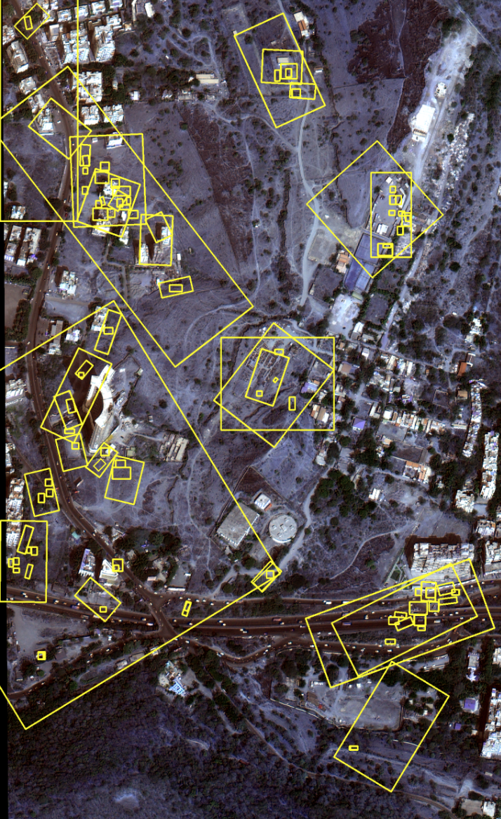
Bounding Box and Location Detection:
This is required to pinpoint the location of construction and the probable area of the site. A series of steps are taken to achieve bounded boxes around built-up structures. Using the heatmap obtained above, first we generate all the countours for all level starting from 1 to 7. Then we find the mapping of related contours such if centroid of a higher level contour is found in the lower level contour then those locations are related. On iteratively creating these maps we get a heirarchy of all the levels of contours. On filtering the areas such that they must have atleast one area with level 3 confidence we achieve a reasonable amount of probable contruction areas.